
Two-Way ANOVA
- Marek Vavrovic
- Jun 14, 2020
- 7 min read
Updated: Jun 20, 2020
A two-way ANOVA test is a statistical test used to determine the effect of two nominal predictor variables on a continuous outcome variable. ANOVA stands for analysis of variance and tests for differences in the effects of independent variables on a dependent variable.
An ANOVA test is the first step in identifying factors that influence a given outcome. Once an ANOVA test is performed, a tester may be able to perform further analysis on the systematic factors that are statistically contributing to the data set's variability. A two-way ANOVA test reveals the results of two independent variables on a dependent variable. ANOVA test results can then be used in an F-test on the significance of the regression formula overall.
Assumptions for ANOVA
To use the ANOVA test we made the following assumptions:
Each group sample is drawn from a normally distributed population
All populations have a common variance
All samples are drawn independently of each other
Within each sample, the observations are sampled randomly and independently of each other
Factor effects are additive
The presence of outliers can also cause problems. In addition, we need to make sure that the F statistic is well behaved. In particular, the F statistic is relatively robust to violations of normality provided:
The populations are symmetrical and uni-modal.
The sample sizes for the groups are equal and greater than 10
In general, as long as the sample sizes are equal (called a balanced model) and sufficiently large, the normality assumption can be violated provided the samples are symmetrical or at least similar in shape (e.g. all are negatively skewed). The F statistic is not so robust to violations of homogeneity of variances. A rule of thumb for balanced models is that if the ratio of the largest variance to smallest variance is less than 3 or 4, the F-test will be valid. If the sample sizes are unequal then smaller differences in variances can invalidate the F-test. Much more attention needs to be paid to unequal variances than to non-normality of data.
Two Factor ANOVA without Replication
Example 1
A new fertilizer has been developed to increase the yield on crops, and the makers of the fertilizer want to better understand which of the three formulations (blends) of this fertilizer are most effective for wheat, corn, soy beans and rice (crops). They test each of the three blends on one sample of each of the four types of crops. The crop yields for the 12 combinations are as shown in Figure 1.

There are two null hypotheses: one for the rows and the other for the columns.
The null hypothesis says that all the blends are same. F statistic for rows = 12.826, f critical = 5.14. Because 12.826 > 5.14 we have to reject the null hypothesis that all the blends are equal. Also, P-value is less than the significance level. If p is low the null must go. Differences between the fertilizer are statistically significant.

Example 2
Let’ assume that McDonald's in Czech Republic uses secret quality agents who pretend to be customers to enter a store and document their experience in terms of customer service, cleanliness, and quality. For its locations in the Czech cities of Prague, Brno and Ostrava, McDonald’s has trained 6 quality agents. Each of the 6 agents will be assigned to visit the same store in each of the 3 cities. The visit sequence will be random. We would like to know if a difference in quality agent ratings exists among the cities. Are they all about the same?

The overall mean is 70. Prague and Brno are bellow mean and Ostrava is above. Are theses ratings significantly different or not?

F critical = 4.1
F statistic = 5.5
5.5 > 4.1 Reject the null hypothesis
P values = 0.02 < α [.05] Reject the null hypothesis

Conducting a Two-Way ANOVA with replication in SPSS
Example 3
In this exercise I am using fictitious data. I have 2 independent variables. Duration of cancelation treatment. It has 3 levels: 6,12,18-week. And I have Gender, separate independent variable that has two levels: male & female. And then I have a dependent variable which contains the results of treatment. Lower symptom level indicates fewer symptoms.
We have one dependent variable SymptomLevel and two independent variables.

Click on Plots...
(i) Move Duration on Horizontal Axis. Press Add button.
(ii) Move Gender on Horizontal Axis. Press Add button.
(iii) Move Duration on Horizontal Axis, Gender on Separate Lines, press Add button and then continue button.

In the Univariate window click on Post Hoc...
We are going to do post hoc test for Duration variable because it has 3 levels. I pick R-E-G-W-Q. You can also try LSD or Tukey or any other test.

We have a look on Estimated Marginal Means under EM Means … button.
Confidence interval adjustment: Bonferroni.

In Options tick Descriptive statistics, Estimates of effect size, Homogeneity tests. Click on the Continue button and then OK to run the tests.

Between - Subjects Factors:
We have 3 levels for duration and 2 levels for gender. The sample sizes are identical for all the different levels of duration and gender.
Descriptive Statistics:
You can have look on the means 6,12,18-week by Gender. Couple of the scores stand out. It is 18-week for Male. That is a low mean score 36. 18-week total is also low. On 12-week Female has significantly lower mean score than Male.

Based on this test we would reject the null hypothesis

Tests of Between-Subjects Effects
Duration: Sig. 0.009: statistically significant difference on the dependent variable SymptomLevel for the independent variable Duration.
Partial Eta Squared: 0.105 means 10.5% of the variance in the dependent variable can be attributed to Duration.
Gender: Sig. 0.894: statistically not significant differences between genders. No difference on the SymptomLevel by Gender.
Partial Eta Squared: 0.000. SymptomLevel variable cannot be explained by gender.
Duration*Gender: Sig. 0.000, Interaction between Duration and Gender is statistically significant. Effect size is 0.281. 28.1% of SymptomLevel can be explained by this interaction. If the lines cross, we should stop right there. Data interpretation is difficult because we cannot say if there is an upwards or downward pattern.

Duration, Estimates: we have low mean for 18-week treatment. We can say that 18-week treatment reduces the number of symptoms.

We know there is a statistically significant difference between the levels of the duration and dependent variable on the symptom level from Test Between-Subjects Effects. Duration Sig. is 0.009. Means there are significant differences between the weeks of treatment. Pairwise Comparison can tell us where this is happening.
We do not have a statistically significant difference between 6-week and 12-week variable [Sig. 1.000]. But we do have significant difference between 6-week and 18-week [Sig. 0.012]. The other scores are statistically not significant because are above 0.05.

The differences between genders are not statistically significant.

Duration: 18-week treatment seems to be much more effective than the other weeks in terms of removing symptoms.

At the 6-week level for male and female the symptom level was roughly the same. For the 12-week program the male symptoms level was higher female was lower, means female was responding better. For the 18-week, female symptoms increase male symptoms show a market decrease in the symptom level. Female benefits from 12-week, male benefits from 18-week treatment.

Conducting a Two-Way ANOVA with replication in Excel
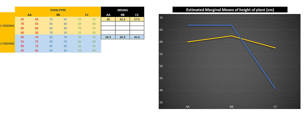
You are a researcher interested in the effectiveness of 3 different cotton plant foods: Awesome Advantage (AA), Big Buds (BB), and Copious Cotton (CC). Therefore, you design an experiment in which you will test each plant food with two feedings per day for 75 days after planting. 8 plants will be tested for each combination. The variable of interest is the plant height in centimetres.
Is there any difference in plant growth when comparing 1 feeding to 2 feedings per day? (feeding frequency). Do some plant foods work better once per day and others better at twice per day? (feeding frequency together with food type).

We are going to perform a test for outliers, normality, homoscedasticity, or homogeneity of variance, we will be visually inspecting the charts. Let's start with homoscedasticity and boxplot.
If we have a look on the interquartile range, we can see these are not too close to each other. The variances are unequal. This is called heteroskedasticity (or heteroscedasticity). It happens when the standard errors of a variable, monitored over a specific amount of time, are non-constant. We can also look on the outliers. You can see there is no score bellow or above any of the whiskers.

We try to evaluate normality now. We can have a look on Histogram or run Descriptive Statistics test to get an idea if the data are normally distributed or not.
As we can see Excel is give us Kurtosis and Skewness values which are relatively close to zero what suggest that the data tails off appropriately and are relatively symmetrical. If we have a look on mean and median values these are close to each other as well. These descriptive statistics values are consistent with a normal distribution.

In the beginning we had couple of questions. For AA, BB, CC, how many feedings produce more growth? Do two feedings produce more growth across ALL plant foods consistently? It appears that two feedings [blue line] are better for AA and BB but not for CC . This type of situation is called an interaction. An interaction occurs when the effect of one factor changes for different levels of the other factor. In this case, the most effective feeding frequency changes across plant food types. On a marginal means graph, as a rule, we look if the lines cross or “would” cross. According the chart we have a significant interaction here, means our 2 factors are too tied together to look at them individually.
Conducting a Two-Way ANOVA with replication in Excel.

Anova table. The first row to interpret is called Sample. This is one feeding versus two feedings per day. F value is lower than F critical means both feedings are equal. We would fail to reject the null hypothesis because the p-value is 0.45 > α=0.05
Columns are the plants [AA, BB,CC]. F value is greater than F critical. The plants are not equal, there are statistically significant differences between the plants. We would reject the null hypothesis and say that each plant reacts differently during the feedings.
Interaction. If the P value is lower than α=0.05 means interaction is statistically significant. When considering one feeding and two feedings per day and its relationship to the plant types there are significant differences.

Comments